The UW Colleges are a unique feature of the public higher education landscape. They are classified as “Associate’s: High-Transfer, High-Traditional” colleges, meaning they largely serve traditional-aged students (coming directly out of high school) with a goal of improving transfer from Associate’s to Bachelor’s degree programs.

Nationwide, there are about 160 of these colleges* and they enroll about 1.5 million undergraduates. Since the end of the Great Recession, enrollments have dropped and today’s enrollments are higher than the pre-Recession levels.^

Colleges located in Midwestern states are experiencing similar enrollment declines since 2010, and the following chart shows the four largest Midwestern Higher Education Compact states’ total enrollments for their “high-transfer, high-traditional” Associate’s degree granting colleges:

Using the UW System’s Accountability Dashboard, we can see how UW Colleges’ enrollment levels have changed relative to four-year universities in the system (this chart excludes UW-Madison and UW-Milwaukee). Approximately 12,000 students enrolled during the fall of 2016-17.**

UW Colleges enrolled approximately 7 percent of the system’s total undergraduates in 2016-17 and this share has hovered between 6 and 8 percent over time.

And a growing share of UW Colleges’ enrollments are from students who identify as Black, Hispanic, or Native American. Since 2010, the percentage of students classified into these three racial/ethnic groups has doubled within the UW Colleges.

As conversations about UW Colleges continue, it is also worth stating these two-year institutions serve different missions than the Wisconsin Technical College System (WTCS). To oversimplify the difference, technical colleges are focused more on vocational training while UW Colleges focuses more on transfer. Nevertheless, the final chart uses IPEDS enrollment data to summarize how enrollments in the technical colleges, university system, and UW Colleges have changed over time.

Notes:

* A “college” could include multiple campuses. For example, UW Colleges is reported as a single institution in IPEDS, but accounts for 13 campuses and an online presence.

^ In all charts, we would get slightly different enrollment trends when using 12-month headcounts from IPEDS, but I used fall enrollment (undergraduate total, degree-seeking and non-degree-seeking).

** Note the axis scale on the previous chart makes the recent enrollment drop look less steep and the prior (IPEDS) data only includes 2015 enrollment, not 2016.

Below are two ways to display the same data.

The first is a trusty old pie chart.

The second is its cooler pastry cousin, the waffle chart.

These data are from IPEDS, just a quick count of public college undergraduates by their college’s selectivity.

We can see in both charts the majority enroll in open-access colleges. But the waffle is easier on the eye, I think.

Turns out, the choice between pies and waffles can be contentious.

If you’re like me, you probably want to use a waffle chart to display your data sometime.

You can make one of these in R using the “waffle” command…if you are familiar with that program. I, sheepishly, am not.

For those of us still in the old school, I made this waffle chart in Excel. Please feel free to use in your own work, but keep in mind this will only work for up to four slices of pie.

Download this Excel file: waffle template

Step one: Enter up to four category names in cells B3:B6

Step two: Enter percentages (high to low) in cells C3:C6. The template is just filling these with random numbers as a placeholder.

Step three: Choose which chart you like better, the square waffle or the rectangle waffle. Both charts link to the same data.

Note: You’ll see two other tabs in this file, “chart 1” and “chart 2,” which are the underlying formulas driving the chart. Just pretend they’re not there.

I created and modified this based on a helpful guide found here. If you end up using this file, please let me know if you detect any bugs. I think I’ve worked them out, but don’t hesitate to contact me if you see any or have suggestions.

Tennessee began implementing performance-based funding in 2011 as part of its statewide effort to improve college completions. The figure below uses IPEDS completion data plotting the average number of bachelor’s degrees produced by each of the state’s 9 universities over time.

One could evaluate the policy by comparing outcomes in the pre-treatment years against those in the post-treatment years. Doing so would result in a statistically significant “impact,” where 320 more students graduated after the policy was in effect.

	Pre	Post	Difference
Tennessee	1940	2260	320

This Interrupted Times Series approach was recently used in a report concluding that 380 more students (Table 24) graduated because of the policy. My IPEDS estimate and the one produced by the evaluation firm use different data, but are in the same ballpark.

Anyway, simply showing a slope changed after a certain point in time is not strong enough evidence to make causal claims. In very limited conditions can one make causal claims with this approach. But this is uncommon, making interrupted time series a pretty uncommon technique to see in policy research.

A better approach would add a comparison group (a la Comparative Interrupted Time Series or its extensions). If one were to do that, then they would compare trends in Tennessee to other universities in the U.S. The graph below does that just for illustrative purposes:

By adding a comparison group, we can see that the gains experienced in Tennessee were pretty much on par with trends occurring elsewhere in the U.S.:

	Pre	Post	Difference
Tennessee	1940	2260	320
Other states	1612	1850	238
Difference	328	411	83

The difference-in-differences estimate, which is a more accurate measure of the policy’s impact, is 83. And if we run all this through a regression model, we can see if 83 is a significant difference between these groups.

It is not:

Using this more appropriate design would likely yield smaller impacts than those reported in the recent evaluation. And these small impacts likely wouldn’t be distinguishable from zero.

I wanted to share this brief back of the envelope illustration for two reasons. First, I am working on a project examining Tennessee’s PBF policy and the only “impact” we are seeing is in the community college sector (more certificates). We are not finding the same results in associate’s degree or bachelor’s degree production. Second, it gives me an opportunity to explain why research design matters in policy analysis. I don’t pretend to be a methodologist or economist; I am an applied education researcher trying my best to keep up with social science standards. Hopefully this quick post illustrates why that’s important.

Below is a summary of high school FAFSA filing up to June 30 for the current and prior filing cycles.

June 30, 2016: 1,949,067
June 30, 2017: 2,128,524

This is a 9% boost in filing, or 179,457 more filers than last year!

You can download the raw data here or below.

We haven’t yet taken a close look at which high schools have shown the most growth, and I won’t pretend to know what these schools did to boost completions, but below is a quick look at the Top 20 in terms of largest raw number increase in FAFSAs. Way to go, Northside High School in Houston, TX, which saw the biggest jump in completions – going from 25 to 457!

	State	School Name	City	June 30 completions (16-17)	June 30 completions (17-18)	Change	Percent Change
1	TX	NORTHSIDE HIGH SCHOOL	HOUSTON	25	457	432	1728%
2	PA	PENN FOSTER HS	SCRANTON	911	1213	302	33%
3	FL	CYPRESS CREEK HIGH	ORLANDO	295	499	204	69%
4	IL	LINCOLN-WAY EAST HIGH SCHOOL	FRANKFORT	327	529	202	62%
5	FL	TIMBER CREEK HIGH	ORLANDO	396	572	176	44%
6	TX	ALLEN H S	ALLEN	674	842	168	25%
7	NC	ROLESVILLE HIGH	ROLESVILLE	95	258	163	172%
8	FL	WILLIAM R BOONE HIGH	ORLANDO	304	467	163	54%
9	CA	WARREN HIGH	DOWNEY	556	710	154	28%
10	CA	RANCHO VERDE HIGH	MORENO VALLEY	465	614	149	32%
11	IL	JONES COLLEGE PREP HIGH SCHOOL	CHICAGO	226	374	148	65%
12	FL	OLYMPIA HIGH	ORLANDO	318	460	142	45%
13	FL	FREEDOM HIGH	ORLANDO	374	515	141	38%
14	NY	NEW UTRECHT HIGH SCHOOL	BROOKLYN	372	511	139	37%
15	NY	BRENTWOOD HIGH SCHOOL	BRENTWOOD	491	630	139	28%
16	TX	THE WOODLANDS H S	THE WOODLANDS	419	555	136	32%
17	PA	PHILADELPHIA PERFORMING ARTS CS	PHILADELPHIA	7	142	135	1929%
18	TX	LOS FRESNOS H S	LOS FRESNOS	341	476	135	40%
19	UT	COPPER HILLS HIGH	WEST JORDAN	256	390	134	52%
20	CA	VALENCIA HIGH	VALENCIA	318	449	131	41%

And in Wisconsin, here’s a list of the Top 20 schools in terms of raw growth in completions:

	State	School Name	City	June 30 completions (16-17)	June 30 completions (17-18)	Change	Percent Change
1	WI	KING INTERNATIONAL	MILWAUKEE	201	278	77	38%
2	WI	BADGER HIGH	LAKE GENEVA	148	217	69	47%
3	WI	OCONOMOWOC HIGH	OCONOMOWOC	194	262	68	35%
4	WI	SUN PRAIRIE HIGH	SUN PRAIRIE	238	306	68	29%
5	WI	CASE HIGH	RACINE	160	227	67	42%
6	WI	EAST HIGH	APPLETON	170	235	65	38%
7	WI	REAGAN COLLEGE PREPARATORY HIGH	MILWAUKEE	206	269	63	31%
8	WI	RIVERSIDE HIGH	MILWAUKEE	183	243	60	33%
9	WI	MIDDLETON HIGH	MIDDLETON	239	296	57	24%
10	WI	DE PERE HIGH	DE PERE	180	235	55	31%
11	WI	BAY PORT HIGH	GREEN BAY	232	281	49	21%
12	WI	FRANKLIN HIGH	FRANKLIN	229	277	48	21%
13	WI	NORTH HIGH	WAUKESHA	119	166	47	39%
14	WI	HAMILTON HIGH	MILWAUKEE	128	174	46	36%
15	WI	EAST HIGH	MADISON	173	218	45	26%
16	WI	CENTRAL HIGH	SALEM	134	178	44	33%
17	WI	CENTRAL HIGH	LA CROSSE	128	171	43	34%
18	WI	MUSKEGO HIGH	MUSKEGO	220	263	43	20%
19	WI	WAUNAKEE HIGH	WAUNAKEE	154	193	39	25%
20	WI	WEST HIGH	WAUKESHA	149	188	39	26%

We will continue to analyze this data and plan to merge with other data sources to gain a better understanding of the variation that exists in filing rates.

We want to be sure to make this data available along the way, so please feel free to download and use the following high school and state-level data comparing the two cycles: FAFSA completions to June 30.xlsx

I wish I had time and resources to make this data more user-friendly and to share more widely. But until then, hopefully this good old fashioned Excel file is of use!

This post provides a new way to import and manage College Scorecard data in Stata.

Alan Riley, Stata’s VP for software development, created the following code that creates the same panel as described in my previous post.

But this one gets the job done in about 15 minutes!

Alan reached out after reading my previous post and seeing some of our Twitter conversation. He didn’t like hearing how long it took me (and others) to run this. So, Alan took it as a challenge to figure out a better way.

And that he did!

I asked if I could share this code here on my blog and he eagerly agreed. He offered one comment for users:

Just one caveat:

I feel that I just made some quick tweaks to the code, and there are probably not only more optimizations that could be found, but it could also be made more robust to potential problems with more use of Stata’s -confirm- and -assert- commands in various places to ensure everything is as expected.

Nick Cox (yes, the same Nick Cox from the Stata Forum) also reached out with some suggestions on the -destring- command I was previously using. I was destringing a lot of unnecessary items, which Alan fixed and greatly speeds up the process. Kevin Fosnacht offered all the labeling code in the previous post. And Daniel Klasik noted some quirks between Mac and PC users, where the “unitid” variable may create an error for Mac users. Thanks, guys!

And here is a .do file where I copied and pasted Alan’s original code (updated 11/14/2017): https://uwmadison.box.com/s/wo6dtfp141x103cen3uq2zr8s09av610

This post provides Stata commands to create a panel dataset out of the College Scorecard data. The first steps take only a few minutes, then the final destring step takes quite a while to run (at least an hour).

Step 1: Download the .csv files from here

In this example, I download these files into a “Scorecard” folder located on my desktop.

Notice how the file names have underscores in them. The first file is titled “MERGED1996_97_PP” and so on. Let’s drop the underscore and number in between (“_97_”) so the file now is titled “MERGED1996PP” and do this for each file:

Step 2: Convert .csv files to .dta files

Our raw data is now downloaded and prepped. Open a Stata .do file and import these .csv files. The following loop is a nice way to do this efficiently:

• Row 2 tells Stata where to find the raw .csv data.
• Row 5 tells Stata to remember (as “i”) any number that fall between 1996 and 2014.
• Row 6 tells Stata to import any .csv file in my directory named “MERGED`i’PP” — here the `i’ is replaced by the numbers 1996 through 2014. This is why we got rid of the underscores in Step 1, it helps this loop operate efficiently.
• Row 7 generates a new variable called “year” and sets its value equal to the corresponding year in the file.
• Row 8 saves each .csv file as a .dta file and keeps the same file naming convention as before.
• Row 9 tells Stata to start anew after each year so we end up with the following files in our directory:

Notice the .dta files are all now here and named in the exact same way as the original .csv files (well, technically I added an underscore after “MERGED”). This loop takes a few minutes to run.

Step 3: Append each year into a single file

Now that we have individual files, we want to stack them all on top of each other. We have to start somewhere, so let’s open the 1996 .dta file and then append all future years, 1997 through 2014, onto this file:

We will do this in a small loop this time, where:

• Row 13 tells Stata to open the 1996 .dta file
• Row 14 tells Stata to remember as “i” the numbers 1997 to 2014
• Row 15 tells Stata to append onto the 1996 file each .dta that corresponds with the year `i’. The “force” command is needed here only because some years a variable is coded as a string and others numeric, so this just tells Stata to bypass that quirk.

Step 4: Destring the data

The data is now in a panel format, where each row contains a unique institution and year. Let’s take a quick look at UW-Madison (unitid=240444) by using the following command:

br ïunitid year instnm  debt_mdn if ïunitid==240444

We’re almost done, but notice a couple of quirks here. First, the median debt value is red, meaning it is string (because 1996 is “NULL”). Second, the variable ïunitid should be renamed to just plain old “unitid” – otherwise, things look pretty good here in terms of setting up a panel.

The following loop will clean this all up for us. It took me at least an hour, be warned. (Thank you Nick Cox for your helpful de-bugging!)

• Row 19 renames ïunitid to unitid
• Row 20 tells Stata to find string variables
• Row 21 tells Stata to remember as “x” all variables in the file
• Rows 22 and 23 replace all those NULLs and PrivacySuppressed cells with “.n” and “.p” missing values, respectively.
• Row 25 destrings and replaces all variables

So now when we look at UW-Madison, we see the median debt values are black, meaning they are destringed (destrung?) with the “NULL” value for 1996 missing.

Step 5: Add variable and value labels

Thanks to Kevin Fosnacht (Indiana University), you can also add labels with the commands found below in the .do file. Thanks, Kevin!

Step 6: Save the new file so you don’t have to run all this again.

You now have all Scorecard data from 1996 to 2014 in a single panel dataset, allowing you to merge with other data sources and analyze this with panel data techniques.

There are several other ways one could go about managing this dataset and creating the panel, so forgive me for any omissions or oversights here. My goal is to simply help remove a data access barrier to facilitate greater research use of this public resource. Grad students developing their research programs might find this a useful data source for contributing to and extending higher education policy scholarship.

.do file: scorecard

Update 6/12/2017: the “.n” and “.p” command had a small bug on the destring loop. But thanks to Nick Cox, this is now fixed! Also, Kevin Fosnacht was so kind as to share his relabeling code, many thanks!

We are 36 weeks into the 2017-18 FAFSA cycle and 2.04 million high school seniors have completed the form as of June 2, 2017. This is an increase of about 200,000 over last cycle, or about a 10% overall increase:

In this chart, a few important spikes stand out. The first is the holiday bumps we see in November and December, where filing slows down in a couple of weeks and the rebounds after the new year. The second is the March bump, as several states (notably, CA) have filing deadlines. The third is an early April bump that is simply an artifact of the way the Office of Federal Student aid began defining a high school senior. Up to that week, seniors included students no older than 18. Now it includes students no older than 19. This is a good change in the long-run, but ideally we would have 18-year-olds reported for the entire cycle.

With these details in mind, below is a chart showing the same trend but for each individual state (to June 2, 2017):

To put this another way, here’s a map showing the percent change in the two cycles, where Utah grew the most (39% increase) and Rhode Island the least (6% decrease).

 

Raw data (.xlsx): State Weeks – Oct to June 2

 

On April 13, 2017, the Wisconsin Assembly Committee on College and Universities held an informational hearing on outcomes-based funding for higher education. The video of the entire hearing is available here. Below are the notes from my testimony, including appendices with additional information.

1. Preliminaries

When approaching PBF/OBF, I think first about the underlying problem to be solved and how PBF gives policymakers the levers to solve them. This approach will hopefully help us avoid predictable pitfalls and maximize the odds of making a lasting and positive difference in educational outcomes.

• What is the underlying problem to be solved/goal to be achieved?
  
  • Some possibilities:
    • Increase number degrees awarded (see Appendix A)
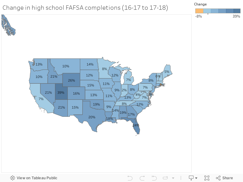
    • Tighten connection between high school and college
    • Close inequalities in graduation rates
    • Improve affordability and debt burdens
    • Improve transparency and accountability for colleges
    • All of the above, plus more?
• What policy levers does PBF/OBF offer for solving these problems?
  • Financial incentives: 2% of UWS annual budget; millions for campuses
  • Persuasive communication: transparency and focusing of goals
  • Capacity building: technical and human resources to perform
  • Routines of learning: system-wide network of best practices, data sharing

• What can we learn from outside higher education?
  • Pay-for-performance should work when:
    • Goals are clearly measured
    • Tasks are routine and straightforward
    • Organizations are specialized, non-complex
    • Employees are not motivated
    • Outcomes are immediately produced
  • But efforts rarely produce large or sustained effects:
    • K-12
    • Job training
    • Crime & policing
    • Public health
    • Child support
  • We are left with a conundrum where the policy is spreading but without convincing or robust evidence that it has improved outcomes: PBF/OBF states have not yet out-performed others.
    • Political success versus programmatic success.

2. Overview of higher education PBF/OBF research
Disentangling the effect of the policy from other noise is challenging, but possible. I have produced some of this research and am the first to say it’s the collection of work – not a single study – that can explain what is happening. Here is a quick overview of the academic evaluations that adhere to social science standards, passed peer review, and are published in the field’s top research journals.

• What are the biggest challenges to doing research in this area?
  • Treatment vs. dosage
  • New vs. old models
  • Secular trend vs. policy impact
  • Lags and implementation time
  • Intended vs. unintended outcomes
• What has the research found?
  • Older studies
    • Documenting which states and when (1990-2010)
    • Focus on AAs and BAs
    • No average effects
      • Small (0.01 SD) lagged effect for BA degrees (PA)
      • Small (0.04 SD) lagged effects for AA (WA)
    • Newer studies
      • Institution-level and state case studies
      • Focus on retention, certificates, AAs, BAs, and resource allocation
      • Account for implementation lags and outcome lags
      • Differentiates old from new models
      • No average effects
        • No effect on graduation rates
        • No effect on BA even with lags (PASSHE, OH, TN, IN)
        • No effect on retention or AA (WA, OH, TN)
        • Modest change in internal budget, research vs instruction
      • Negative effects
        • Sharp increase in short-term certificates (WA, TN)
        • Reduced access for Pell and minority students (IN)
        • Less Pell Grant revenue

3. Pros and cons

• Despite these findings, there is still an appetite for adopting and expanding PBF/OBF in the states and for good reason:
  • Focus campus attention on system-wide goals
  • Increases public transparency
  • Helps stimulate campus reform efforts
    • Remedial education reform
    • Course articulation agreements
    • More academic advisors, tutors, etc.

• But pursuing this course of action has significant costs that should be considered and avoided to the fullest extent possible:
  • Transaction costs: new administrative burdens for campuses
  • Goal displacement: trades research for teaching, weaker standards
  • Strategic responses: gaming when tasks are complex and stakes are high
  • Democratic responsiveness: formula, not legislators, drive the budget
  • Negativity bias: focus on failures over successes, can distract attention

4. Recommendations

If I were asked to design a PBF/OBF system for the state, I would adhere to the following principles. These are guided by the most recent and rigorous research findings in performance management and higher education finance:

• Use all policy instruments available to maximize chances of success.
  • Financial capacity (e.g., instructional expenses and faculty-student ratio) is the strongest predictor of time-to-degree, so reinvestment will likely yield greatest results regardless of funding model
  • Analytical capacity and data infrastructure needs to be built, used, and sustained over time to make the most of the performance data generated by the new model
  • Invest in system’s capacity to collect, verify, and disseminate data (see Missouri’s Attorney General’s recent audit)
  • Build campus’ technical and human resource capacity before asking campuses to reach specific goals (Appendix B has promising practices).

• Avoid one-size-fits-all approaches by differentiating by mission, campus, and student body.
  • Different metrics per campus
  • Different weights per metric
  • Input-adjusted metrics
  • Hold-harmless provisions to navigate volatility
• Use prospective, rather than retrospective, metrics to gauge progress and performance on various outcomes.
  • Consider developing an “innovation fund” where campuses submit requests for seed funding allowing them to scale up or develop promising programs/practices they currently do not have capacity to implement.
  • Use growth measures rather than peer-comparisons, system averages, or rankings when distributing funds.
  • Monitor and adjust to avoid negative outcomes and unintended results.

• Engage campuses and other stakeholders in developing and designing performance indicators. Without this, it is unlikely for PBF/OBF to be visible at the ground-level and to be sustained over political administrations.
  • Create a steering committee to solicit feedback, offer guidance, and assess progress toward meeting system PBF/OBF goals.
  • See Appendix C for questions this group could help answer.

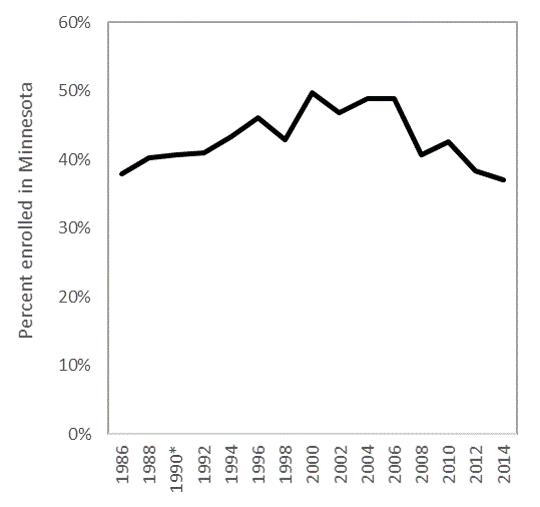
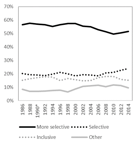
Appendix A:
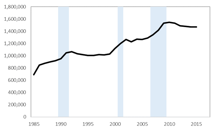
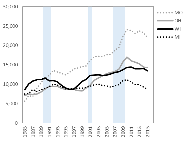
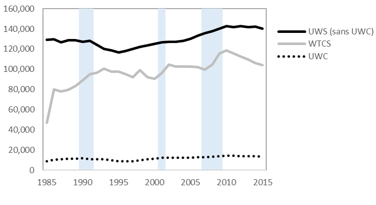
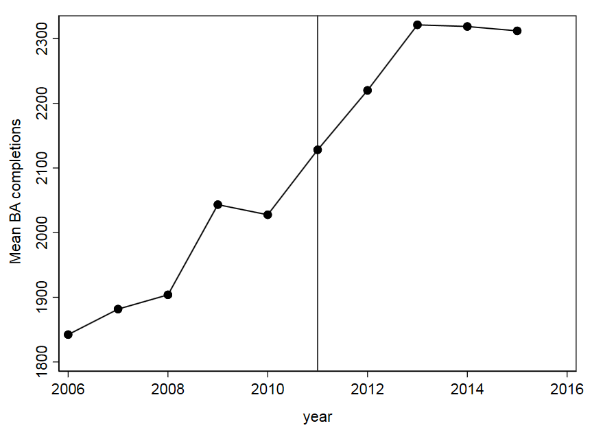
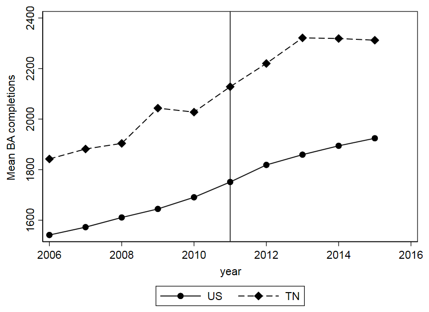
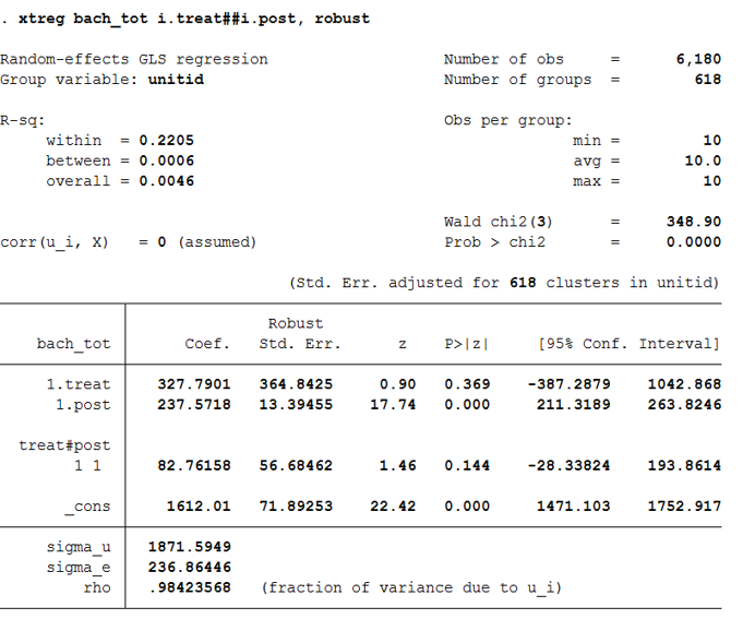
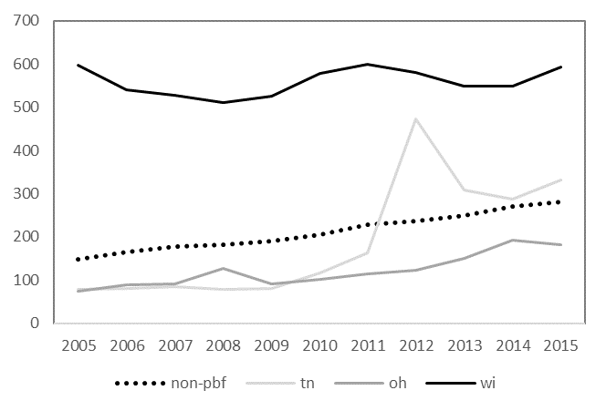
On average, PBF/OBF states have not yet outperformed non-PBF/OBF states in terms of degree completions. To the extent they have, the effects are isolated in short-term certificate programs, which do not appear to lead to associate’s degrees and that (on average) do not yield greater labor market returns than high school diplomas.

Figure 1:
Average number of short-term certificates produced by community/technical colleges

Figure 2:
Average number of long-term certificates produced by community/technical colleges

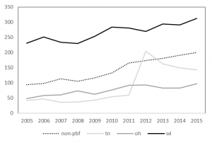
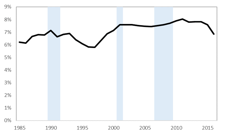
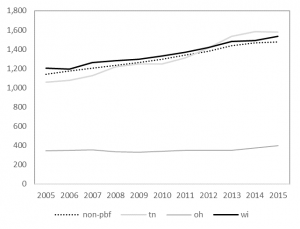
Figure 3:

Average number of associate’s degrees produced by community/technical colleges

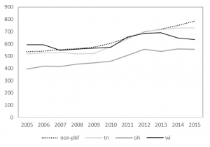
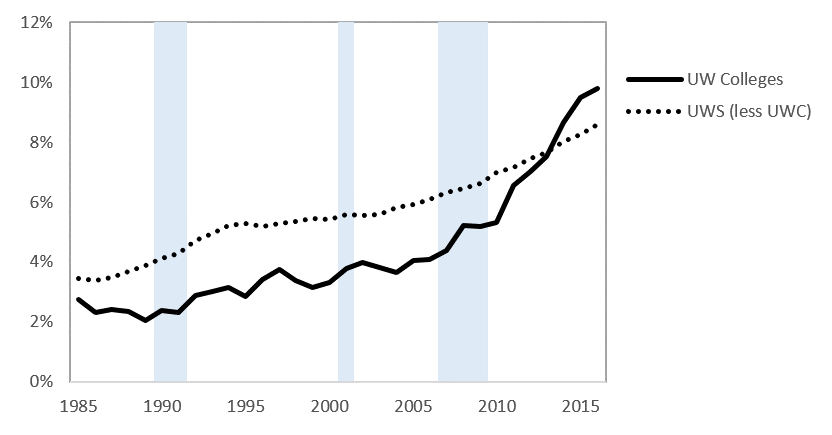
Figure 4:
Average number of bachelor’s degrees produced by public research universities

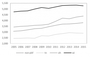
Figure 5:
Average number of bachelor’s degrees produced by public masters/bachelor’s universities

Appendix B:

While there are many proposed ideas to improve student outcomes in higher education, most are not evidence-based. This policy note identifies practices where there is a strong evidence base for what works, based on the high-quality, recent and rigorous research designs.

• Investment in instructional expenditures positively impacts graduation rates.[i] Reducing instructional resources leads to larger class sizes and higher faculty-to-student ratios, which is a leading reason why students take longer to earn their degrees today.[ii] When colleges invest more in instruction, their students also experience more favorable employment outcomes.[iii] There may be cost-saving rationales to move instruction to online platforms, but this does not improve student outcomes and often results in poorer academic performance primarily concentrated among underrepresented groups.[iv]
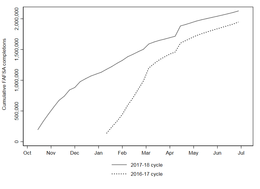
• Outside the classroom, student support services like advising, counseling, and mentoring are necessary to help students succeed.[v] Recent studies have found retention and graduation rates increase by both intensive and simpler interventions that help students stay on track.[vi] Interventions that help students navigate the college application and financial aid process have a particularly strong evidence base of success.[vii]
• Need-based financial aid increases graduation rates by approximately 5 percentage points for each $1,000 awarded.[viii] When students receive aid, they attempt and complete more credit hours, work fewer hours, and have even more incentives to persist through graduation.[ix] Coupling financial aid with additional student support services (e.g., individualized advising) yields even stronger outcomes, [x] particularly among traditionally underrepresented students.[xi] When tuition rises without additional aid, students are less likely to enroll and persist and these effects again disproportionately affect underrepresented students.[xii]
• Remedial coursework slows students’ progress toward their degree, but does not necessarily prevent them from graduating. Remedial completers often perform similar to their peers and these leveling effects are strongest for the poorest-prepared students.[xiii] High school transcripts do a better job than placement exams in predicting remediation success,[xiv] and some positive effects may come via changing instructional practices and delivering corequisite remedial coursework.[xv] But even without reforming remediation, enhanced academic and financial support services have been found to greatly improve remedial completion and ultimately graduation rates.[xvi]
• Place-based College Promise programs guarantee college admission and tuition waivers for local high school students. There are more than 80 programs operating nationwide with several across Wisconsin: Gateway College Promise, LaCrosse Promise, Milwaukee Area Technical College Promise, Milwaukee’s Degree Project, and Madison Promise.[xvii] Program evaluations in Kalamazoo, MI, and Knoxville, TN, find the programs have positive effects on college access, choice, and progress toward degree completion.[xviii]

Appendix C:
Below are additional questions to consider as legislators, regents, and system officials move forward in their planning efforts.

• What is the purpose of PBF and who are the most likely users of the data? Is it external accountability – implying the legislature or public will be the primary users? Or campus-driven improvement – implying campus administration will be the primary users?
• How is the data collected, verified, and reported? By whom and with what guidelines?
• How well does a metric measure what it sets out to measure? Are there key aspects of higher education that are not being measured?
• What technical and human resource capacity do campuses have to use this data? How?
• What unintended result might occur by prioritizing a particular metric over another?
• How might the numbers be gamed without improving performance or outcomes?
• Who on campus will translate the system’s performance goals into practice? How?
• When numbers look bad, how might officials respond (negativity bias)?

Endnotes

[i] Webber, D. A. (2012). Expenditures and postsecondary graduation: An investigation using individual-level data from the state of Ohio. Economics of Education Review, 31(5), 615–618.

[ii] Bound, J., Lovenheim, M. F., & Turner, S. (2012). Increasing time to baccalaureate degree in the United States. Education, 7(4), 375–424. Bettinger, E. P., & Long, B. T. (2016). Mass Instruction or Higher Learning? The Impact of College Class Size on Student Retention and Graduation. Education Finance and Policy.

[iii] Griffith, A. L., & Rask, K. N. (2016). The effect of institutional expenditures on employment outcomes and earnings. Economic Inquiry, 54(4), 1931–1945.

[iv] Bowen, W., Chingos, M., Lack, K., & Nygren, T. I. (2014). Interactive Learning Online at Public Universities: Evidence from a Six‐Campus Randomized Trial. Journal of Policy Analysis and Management, 33(1), 94–111.

[v] Castleman, B., & Goodman, J. (2016). Intensive College Counseling and the Enrollment and Persistence of Low Income Students. Education Finance and Policy.

[vi] Bettinger, E. P., & Baker, R. B. (2014). The Effects of Student Coaching An Evaluation of a Randomized Experiment in Student Advising. Educational Evaluation and Policy Analysis, 36(1), 3–19.

[vii] Bettinger, E. P., Long, B. T., Oreopoulos, P., & Sanbonmatsu, L. (2012). The Role of application assistance and information in college decisions: results from the H&R Block FAFSA experiment. The Quarterly Journal of Economics, 127(3), 1205–1242.

[viii] Castleman, B. L., & Long, B. T. (2016). Looking beyond Enrollment: The Causal Effect of Need-Based Grants on College Access, Persistence, and Graduation. Journal of Labor Economics, 34(4), 1023–1073. Scott-Clayton, J. (2011). On money and motivation: a quasi-experimental analysis of financial incentives for college achievement. Journal of Human Resources, 46(3), 614–646.

[ix] Mayer, A., Patel, R., Rudd, T., & Ratledge, A. (2015). Designing scholarships to improve college success: Final report on the Performance-based scholarship demonstration. Washington, DC: MDRC. Retrieved from http://www.mdrc.org/sites/default/files/designing_scholarships_FR.pdf Broton, K. M., Goldrick-Rab, S., & Benson, J. (2016). Working for College: The Causal Impacts of Financial Grants on Undergraduate Employment. Educational Evaluation and Policy Analysis, 38(3), 477–494.

[x] Page, L. C., Castleman, B., & Sahadewo, G. A. (Feb. 1, 2016). More than Dollars for Scholars: The Impact of the Dell Scholars Program on College Access, Persistence and Degree Attainment. Persistence and Degree Attainment.

[xi] Angrist, J., Autor, D., Hudson, S., & Pallais, A. (2015). Leveling Up: Early Results from a Randomized Evaluation of Post-Secondary Aid. Retrieved from http://economics.mit.edu/files/11662

[xii] Hemelt, S., & Marcotte, D. (2016). The Changing Landscape of Tuition and Enrollment in American Public Higher Education. The Russell Sage Foundation Journal of the Social Sciences, 2(1), 42–68.

[xiii] Bettinger, E. P., Boatman, A., & Long, B. T. (2013). Student supports: Developmental education and other academic programs. The Future of Children, 23(1), 93–115. Chen, X. (2016, September 6). Remedial Coursetaking at U.S. Public 2- and 4-Year Institutions: Scope, Experiences, and Outcomes. Retrieved from https://nces.ed.gov/pubsearch/pubsinfo.asp?pubid=2016405

[xiv] Scott-Clayton, J., Crosta, P. M., & Belfield, C. R. (2014). Improving the Targeting of Treatment: Evidence From College Remediation. Educational Evaluation and Policy Analysis, 36(3), 371–393. Ngo, F., & Melguizo, T. (2016). How Can Placement Policy Improve Math Remediation Outcomes? Evidence From Experimentation in Community Colleges. Educational Evaluation and Policy Analysis, 38(1), 171–196.

[xv] Logue, A. W., Watanabe-Rose, M., & Douglas, D. (2016). Should Students Assessed as Needing Remedial Mathematics Take College-Level Quantitative Courses Instead? Educational Evaluation and Policy Analysis, 38(3), 578–598.  Wang, X., Sun, N., & Wickersham, K. (2016). Turning math remediation into “homeroom”: Contextualization as a motivational environment for remedial math students at community colleges.

[xvi] Scrivener, S., Weiss, M. J., Ratledge, A., Rudd, T., Sommo, C., & Fresques, H. (2015). Doubling Graduation Rates: Three-Year Effects of CUNY’s Accelerated Study in Associate Programs (ASAP) for Developmental Education Students. Washington, DC: MDRC. Butcher, K. F., & Visher, M. G. (2013). The Impact of a Classroom-Based Guidance Program on Student Performance in Community College Math Classes. Educational Evaluation and Policy Analysis, 35(3), 298–323.

[xvii] Upjohn Institute. (2016). Local Place-Based Scholarship Programs. Upjohn Institute. Retrieved from http://www.upjohn.org/sites/default/files/promise/Lumina/Promisescholarshipprograms.pdf

[xviii] Carruthers, C.  & Fox, W. (2016). Aid for all: College coaching, financial aid, and post-secondary persistence in Tennessee. Economics of Education Review, 51, 97–112. Andrews, R., DesJardins, S., & Ranchhod, V. (2010). The effects of the Kalamazoo Promise on college choice. Economics of Education Review, 29(5), 722–737.

Last week, two state lawmakers proposed a new merit-based financial aid program designed to help keep the “best and brightest” Wisconsin students in-state for college. This got me intrigued about the extent of out-of-state migration occurring among recent WI high school graduates: how many students go out of state in the first place?  And where do they go?

To answer the second question first, below is a map showing where recent Wisconsin high school graduates began college:

In answering the first question, here are the out-migration patterns of recent Wisconsin high school graduates since 1986 (Figure 1). During the 1980s and 1990s, the number of WI residents attending college out-of-state steadily rose. After its peak in the early 2000s, the number has steadily fallen over the past decade. In 2014, approximately 7,600 WI high school graduates went out of state for college.

Figure 1:
Number of WI recent high school graduates enrolling outside Wisconsin

The steady drop in out-of-state enrollment coincides with the statewide trend of fewer high school graduates (Figure 2). With fewer students graduating from high school, there are fewer attending out-of-state and we should not expect this trend to reverse any time soon. This chart uses WICHE projections of high school graduates in the state, which is expected to plateau and then decline over the next decade.

Figure 2:
Total number of high school graduates in Wisconsin

With fewer graduates – and fewer leaving Wisconsin – it is the proportion of students leaving that gives a clearer view of out-migration. Figure 3 shows the percentage of recent high school graduates from Wisconsin who enroll in other states. After steady growth in the 1980s, this trend stabilizes in the mid-1990s and has hovered around 17 to 19 percent since then.

Figure 3:
Percentage of recent high school graduates attending out of state

With about 1 in 5 recent high school graduates leaving the state, this puts Wisconsin right at the national average in terms of out-migration. Figure 4 uses Digest of Education Statistics data to show how Wisconsin fares compared to other states. On one extreme is Vermont, where more than half of their recent high school graduates attend out of state. On the other extreme is Mississippi, where fewer than 1 in 10 leave for college. Wisconsin’s out-migration rate is higher than Michigan and Iowa, but far lower than Illinois and Minnesota.

Figure 4:
Percent of recent high school graduates enrolling out-of-state

Since Wisconsin and Minnesota have a tuition reciprocity agreement, the next figure shows the share of Wisconsin out-migrants who attended a college in Minnesota. Not all of out-migrants participate in a tuition reciprocity agreement, so this chart should not be interpreted in that light; rather, this simply shows the proportion of Wisconsin residents who attended any Minnesota institution. In the early 2000s, the majority of Wisconsin leavers went to Minnesota, but this is no longer the case.

Figure 5:
Share of Wisconsin high school graduates enrolled in Minnesota colleges

When Wisconsin high schoolers go out of state for college, they often attend “more selective” four-year universities. For reference, three UW System universities are classified in this category: Madison, Eau Claire, and La Crosse. However, Figure 6 uses the Carnegie Classification to show this is not always the case, as many leavers attend less selective institutions. This trend requires greater attention, but may indicate that students leave the state for other reasons than attending highly-selective universities.

Figure 6:
Percent of recent high school graduates who left Wisconsin, by selectivity band

The purpose of this post is to help contextualize and bring data to bear on recent discussions regarding student migration patterns. These back of the envelope estimates use IPEDS data that include only first-time degree-seeking students who graduated high school within the past 12-months and enrolled in college. It is possible other patterns emerge using different datasets, for Wisconsin residents who are not recent high school graduates, or for those who are not first-time students. Much more research is needed to track the extent of out-migration, but the sketches provided here aim to help explain the extent of out-migration among recent high school graduates and to identify where out-migrants enroll. Knowing this may help diagnose the severity of the “brain drain” problem while also helping campus leaders develop efficient and effective strategies for growing the stock of human capital in the state.

Data:

	Total	Stayed in Wisconsin			Left Wisconsin
		Subtotal	Public 4yr	Non-profit 4yr	Subtotal	Public 4yr	Non-profit 4yr
1986	31,277	28,058	19,069	2,508	3,219	1,356	1,632
1988	33,774	29,268	18,753	3,265	4,506	2,006	2,229
1990*	33,269	28,525	17,037	3,529	4,744	2,071	2,365
1992	32,763	27,782	15,321	3,793	4,981	2,136	2,500
1994	31,771	26,585	15,638	3,367	5,186	2,367	2,438
1996	33,151	27,371	17,330	3,333	5,780	2,599	2,739
1998	34,621	28,592	18,802	3,662	6,029	2,788	2,836
2000	36,661	29,946	17,969	3,851	6,715	3,213	2,909
2002	38,148	31,135	19,046	3,733	7,013	3,526	2,682
2004	39,420	32,040	19,370	4,078	7,380	3,875	2,622
2006	42,270	34,212	21,029	4,528	8,058	3,851	3,173
2008	41,749	33,812	20,546	4,620	7,937	3,721	3,259
2010	42,424	34,366	20,820	4,682	8,058	3,661	3,352
2012	41,945	34,220	21,117	4,337	7,725	3,565	3,262
2014	40,489	32,812	20,502	4,271	7,677	3,598	3,340

* 1990 is estimated by taking the mean of the prior and following years; data are not reported this year.

As of April 21, 2017, just over 1.9 million high school seniors completed the FAFSA. This is about 0.3 million more than at the same week last year, or a nice 15% bump. By the end of June last year, about 1.95 million students filed, so we’re on pace to surpass that number next month.

There is another bump worth keeping track of here. Beginning with the April 14 data release, the US Department of Education started counting 19 year old high school seniors. Prior to that week, all data represented 18 year olds.

On the upside, including 19 year olds now gives us a fuller picture of FAFSA filing. But on the downside, this affects our ability to consistently measure weekly changes for the full cycle. We’re hopeful the good folks at FSA will be able to run this data for 18 year olds and 19 years olds, separately, and we’ll provide updates accordingly.

This bump also occurred around the federal tax filing deadline, so it could also be driven in part by families filing the form when they did their taxes. We would be more likely to see that in last year’s cycle that didn’t have PPY, but we can’t disentangle all that here in our simple trend line. We’re just sharing our top-line trends in filing, see the raw data below:

Week	Calendar	2016-17	2017-18
1	10/1
2	10/7		196,736
3	10/14		328,607
4	10/21		448,958
5	10/28		563,560
6	11/4		672,694
7	11/11		740,843
8	11/18		842,620
9	11/25		882,778
10	12/2		976,563
11	12/9		1,023,711
12	12/16		1,067,470
13	12/23		1,099,324
14	12/30		1,130,204
15	1/6	135,387	1,177,839
16	1/13	239,605	1,223,452
17	1/20	334,837	1,276,410
18	1/27	444,951	1,323,681
19	2/3	591,914	1,382,554
20	2/10	711,858	1,422,119
21	2/17	852,752	1,464,928
22	2/24	990,403	1,504,861
23	3/3	1,198,080	1,589,941
24	3/10	1,269,537	1,622,445
25	3/17	1,332,608	1,649,064
26	3/24	1,380,565	1,669,891
27	3/31	1,425,995	1,693,031
28	4/7	1,458,624	1,716,540
29	4/14	1,604,050	1,883,706
30	4/21	1,645,964	1,908,146