Difference-in-differences is gaining popularity in higher education policy research and for good reason. Under certain conditions, it can help us evaluate the effectiveness of policy changes.

The basic idea is that two groups were following similar trend lines for a period of time. But eventually, one group gets exposed to a new policy (the treatment) while the other group does not (the comparison). This change essentially splits time in two, where the treatment group’s exposure to the policy puts them on a new trend line. Had the policy never been adopted, the two groups would have continued on similar paths.

I made a data file and show the steps I took to conduct this analysis in Stata.

Step 1: Generate treatment variable

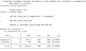
Let’s say College A is exposed to the policy change (treatment) and College B is not (comparison). We just need a simple dummy variable to categorize these two groups. Let’s call it “treat,” where College A gets a value of 1 and College B gets a value of 0.

Step 2: Generate “post” policy variable

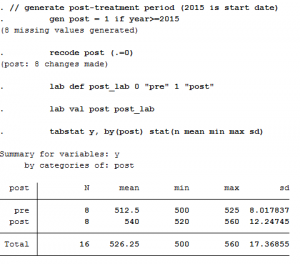
In the previous step, we didn’t say when the policy change occurred, so we need to do that now. Let’s say it began in 2015, meaning all years from that point forward are “post-policy” while those prior are “pre-policy.”

Step 3: Examine trends for the two groups

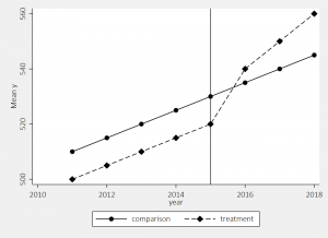
Now that we’ve identified the treatment/control and the pre/post periods, we can put it all together in a simple graph. I like to use the user-written “lgraph” command (use “ssc install lgraph, replace” to get it).

We see here the two groups were following similar trends prior to the 2015 policy change, and then the treatment group started to increase at a higher rate while the comparison group did not.

Step 4: Difference-in-differences means table

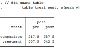
The visual inspection looks like there’s probably a policy effect, but it’s hard to tell the magnitude. To get at that, we need to measure the difference in groups means before and after the policy:

Below is a simple table calculating the difference between the two groups before (-10) and after (5) the policy. It then calculates the difference before and after within each group (20 and 35, respectively).

	Pre	Post	Difference
Comparison	517.5	537.5	20
Treatment	507.5	542.5	35
Difference	-10	5	15

The comparison group increased by 20 units after the policy, while the treatment increased by 35. Similarly, the treatment group was 10 units lower than the comparison group prior to the policy, but was ahead by 5 units after. When we calculate the difference in the group differences, we get 15 (e.g., 35 minus 20, or 5 minus -10).

Step 5: Difference-in-differences regression

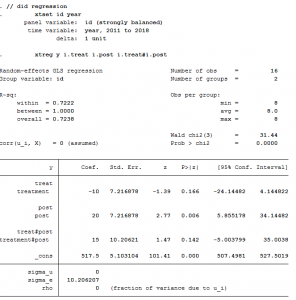
We can run a regression on the data using the two variables created in Steps 1 and 2. The only trick is we need to interact those two variables (treat x post) to get our difference-in-differences estimate.

Here, the “treat” dummy measures the treatment group’s pre-policy difference from the comparison group. And “post” is the comparison groups post-policy change. The interaction between the two variables (“treat x post”) is our average treatment effect of 15, the same number we saw in the previous step. The intercept is the comparison group’s pre-policy mean.

In a regression framework, we can easily add covariates, use multiple comparison groups for robustness checks, and address issues that may arise with respect to standard errors. Doing so can help rule out plausible alternative explanations to the findings, assuming other important considerations are also met.

My goal with this post was to break down the difference-in-differences approach to help make it a little more accessible and less intimidating to researchers/policy analysts. I am still leaning a lot about the technique, so please consider these steps some illustrative tips to get oriented/introduced.

Stata replication code:

// generate treatment variable (College A is the treated unit, College B is comparison)
gen treat = 1 if id==1
recode treat (.=0)
lab def treat_lab 0 “comparison” 1 “treatment”
lab val treat treat_lab
tabstat y, by(treat) stat(n mean min max sd)

// generate post-treatment period (2015 is start date)
gen post = 1 if year>=2015
recode post (.=0)
lab def post_lab 0 “pre” 1 “post”
lab val post post_lab
tabstat y, by(post) stat(n mean min max sd)

// descriptives of the two groups
table year treat, c(mean y)
ssc install lgraph, replace
lgraph y year, by(treat) stat(mean) xline(2015) ylab(, nogrid) scheme(s2mono)

// did means table
table treat post, c(mean y)

// did regression
xtset id year
xtreg y i.treat i.post i.treat#i.post